WP5 — Resilient Networks - Experimental Validation (Final Report)#
Authors
Stephan Kenzelmann, Luca Haab, Fabrizio Sossan — December 12, 2025
1. Introduction#
Microgrids are becoming a vital component of modern power systems, offering localized energy generation and distribution that enhance efficiency, sustainability, and availability. However, microgrids that integrate significant amounts of power-converter-interfaced renewable energy sources may face challenges in maintaining stability and reliable operation, particularly when operating in islanded mode, disconnected from the main grid. To address these challenges and ensure robust performance of low-inertia microgrids, the development and implementation of appropriate control algorithms are essential.
Grid-forming (GFM) converters can provide stable and autonomous operation, as opposed to grid-following (GFL) converters, even without the presence of synchronous generators. Among various control strategies for power converters and distributed generation, droop control is widely used due to its simplicity and effectiveness in achieving power sharing across multiple units. However, droop control alone may not suffice in low-inertia environments, necessitating enhancements to ensure system stability. A well-known enhancement is the integration of virtual inertia into droop control: virtual inertia mimics the behaviour of physical inertia, ensuring stable and reliable operation even under varying load conditions.
This report presents the implementation of a grid-forming control strategy with synthetic inertia in a custom-designed power converter, along with its integration and testing within a microgrid characterized by low and zero physical inertia. We provide experimental results that highlight the electromechanical interactions between real and virtual inertia, and demonstrate how synthetic inertia can be tuned to effectively replicate the behaviour of rotating masses.
2. Experimental setup and methodology#
This section outlines the experimental setup and details the methodology employed for grid-forming control, inertia emulation, and frequency regulation.
2.1 Microgrid topology and configuration#
The experiments presented in this report are conducted in the GridLab laboratory at HES-SO Valais-Wallis, using the Dispatch testbench. This setup is a reduced-scale experimental grid designed to emulate the generation and transmission characteristics of a real-world power system. It features a reconfigurable topology enabled by an array of circuit breakers, along with emulated power lines implemented using discrete components. The system includes power transformers, synchronous generators, prime movers, electrical loads, and general-purpose grid-connection points; these connection points are used in this study to integrate power-converter-interfaced resources.
The system operates as a three-phase system with a line voltage of 400 V RMS. The microgrid can operate in both islanded and grid-connected mode (by connecting to the building’s grid). For the experiments in this report, we use the part of the grid highlighted in Figure 1, which replicates a medium-voltage distribution grid with overhead lines and underground cables.
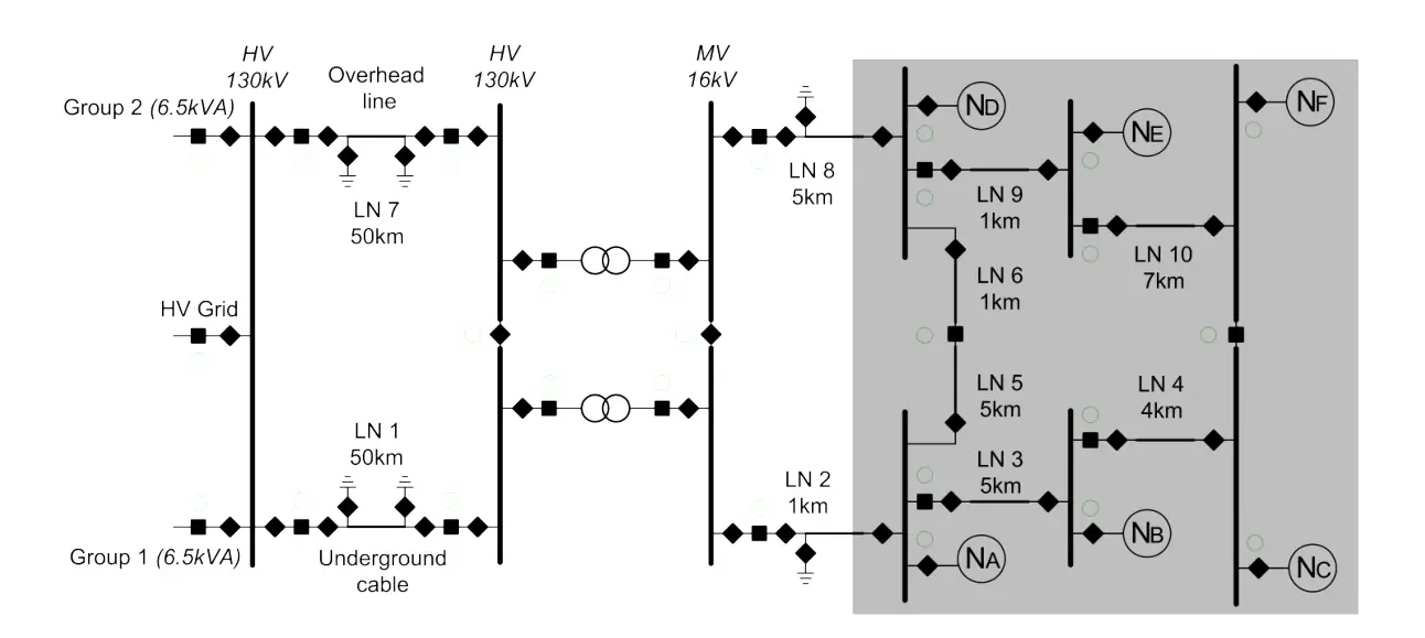 Figure 1: Topology of the “Dispatch” testbench. The considered islanded
microgrid is in the shaded box.
Figure 1: Topology of the “Dispatch” testbench. The considered islanded
microgrid is in the shaded box.
The line lengths are given in the table below; the parameters per unit length of the transversal impedance of the equivalent π model are \(R' = 0.247\ \Omega/\text{km}\) and \(L' = 0.369\ \text{mH/km}\). Loads and power converters are connected to nodes from \(N_A\) to \(N_F\).
| Line | L3 | L4 | L5 | L6 | L9 | L10 |
|---|---|---|---|---|---|---|
| Length | 5 km | 4 km | 5 km | 1 km | 1 km | 7 km |
Table 1: Line lengths.
2.2 Synchronous generators and control#
We employ two 3.5 kVA, 400 V (RMS), 2-pole three-phase synchronous generators, each driven by a prime mover emulated using a brushless motor, to replicate conventional dispatchable synchronous generation. Each generator is equipped with a speed governor implementing droop control, as illustrated in Figure 2. The governor modulates the prime mover’s torque to maintain the generator’s electrical rotational speed at the nominal frequency of 50 Hz. The governor parameters are tuned to meet the timing requirements for primary frequency control. The inertia constant of each generation unit is \(H = 0.467\ \text{s}\).
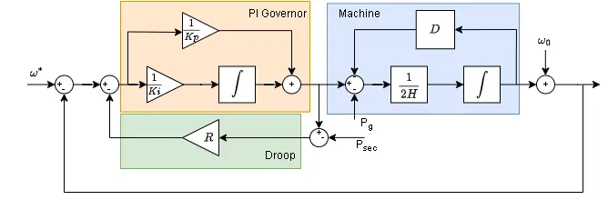 Figure 2: Speed governor of the conventional synchronous generation units.
2.3 AC/DC power converters and control#
The power converters are an in-house developed rapid-prototyping platform (see WP4) designed for a wide range of applications including motor drives and grid converters, aimed at research and educational purposes. This modular system uses 2-level SiC semiconductors and can accommodate up to 10 half-bridges in its maximum configuration.
For control, the system supports either a TI-TMS320F28377S microprocessor or a Typhoon Hardware-in-the-Loop (HIL) system. It is equipped with LCL filter stages, EMI filters, and DC-link precharge stages.
In the current configuration the three-phase converter is managed by the Typhoon HIL system. The DC link of the two converters is powered by a 750 V DC voltage source, emulating a battery energy storage system.
The converter control incorporates droop functionality to enable load sharing among multiple units; droop control is selected for its ability to operate in a decentralized manner without requiring communication, adjusting power and voltage references based on predefined droop coefficients and local voltage and frequency measurements. Additionally, to support grid frequency, the converter implements PLL-free synthetic inertia to emulate the dynamic behaviour of traditional synchronous generators.
The control diagram is shown in Figure 3. A cascade control structure in the dq-coordinates is employed, with a current controller in the inner loop and a voltage controller in the outer loop. Droop control is applied to both active and reactive power: reactive power determines the new setpoint for the d-axis voltage reference, while active power adjusts the converter’s load angle. The implemented inertia influences the mechanical equivalent of the rotating mass and hence the load angle.
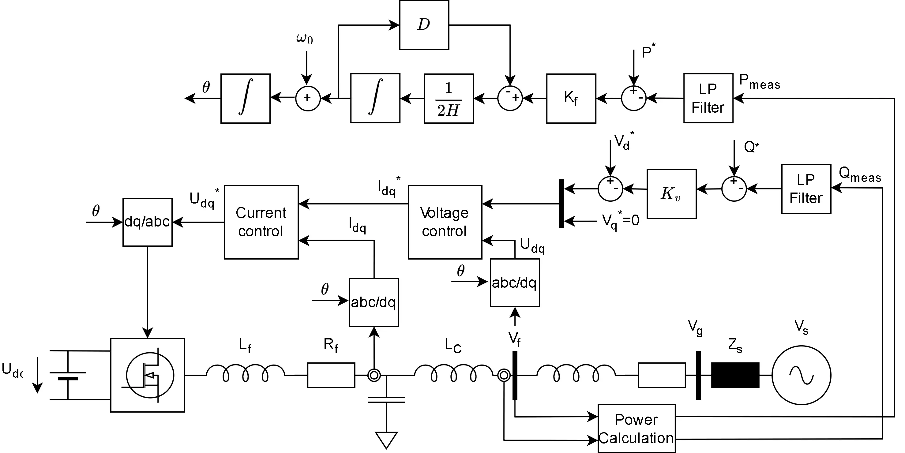 Figure 3: GFM control structure with virtual inertia and droop control.
The synthetic inertia is implemented using the swing equation with damping:
where \(H\) is the inertia constant in seconds, \(\omega\) is the per-unit rotational speed, \(P_m\) is the produced electrical power (in per unit relative to the rated power of the converter), \(P_e\) is the per-unit consumed power, and \(D\) the damping ratio. The inertia constant relates to the moment of inertia \(I\) and the system’s rated power \(S\) by
2.4 Monitoring and control infrastructure#
Nodal voltages and currents within the microgrid are continuously monitored using SICAM-T measurement devices, which provide RMS values at a temporal resolution of 0.1 s. These measurements are logged in a time-series database for later analysis and operational supervision.
Communication between the power converters, generation units, and the Energy Management System (EMS) is facilitated via a Modbus interface over a wired Ethernet network. This communication infrastructure enables dispatching the system; the detailed dispatch strategy lies beyond the scope of the present analysis. The EMS can control the startup and shutdown of the converters and set the active and reactive power references for droop control through Modbus. Additionally, various control parameters — droop coefficients, virtual inertia, damping factors, governor settings — can be configured remotely via the same interface.
 Figure 4: Overview of the experimental setup. The two programmable power
converters are mounted in racks on the right; the synchronous generators are
partially visible in the central part of the picture.
Figure 4: Overview of the experimental setup. The two programmable power
converters are mounted in racks on the right; the synchronous generators are
partially visible in the central part of the picture.
3. Experiments#
3.1 Test conditions#
The microgrid is tested under various configurations, since synchronous generators, GFM converters, and resistive loads can be connected to any node within the system. In addition, the interconnecting lines of the microgrid are reconfigured to empirically assess the impact of different line impedances (long vs. short transmission lines). The nominal power of each converter is 2 kW, while the synchronous generator has a nominal power of 3.5 kW. All converters share the same rated power and droop coefficient; inertia is treated as a tunable parameter and can be varied during experiments.
3.2 No-inertia microgrid with two GFM converters#
In this test, the two converters serve as the sole generation sources within the microgrid. GFM control is applied with virtual-inertia values ranging from 0.01 s to 5 s. A 3.5 kW load step is applied at node \(N_D\).
Two microgrid configurations are tested:
- Scenario 1 — Short distance between converters: nodes \(N_D\) and \(N_F\) separated by 8 km (lines LN 9 and LN 10 active), shown on the left of Figure 5.
- Scenario 2 — Longer line distance of 17 km: converters at \(N_D\) and \(N_A\), separated by lines LN 9, LN 10, LN 4 and LN 3, shown on the right of Figure 5.
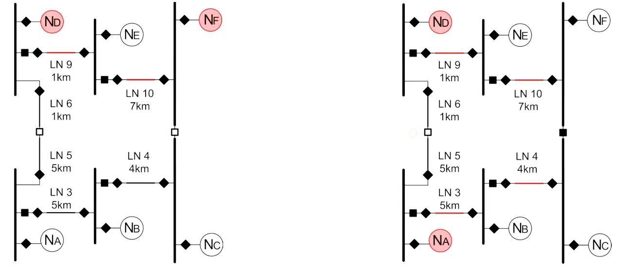 Figure 5: (Left) Scenario 1 — short transmission line distance.
(Right) Scenario 2 — longer transmission line distance.
Figure 5: (Left) Scenario 1 — short transmission line distance.
(Right) Scenario 2 — longer transmission line distance.
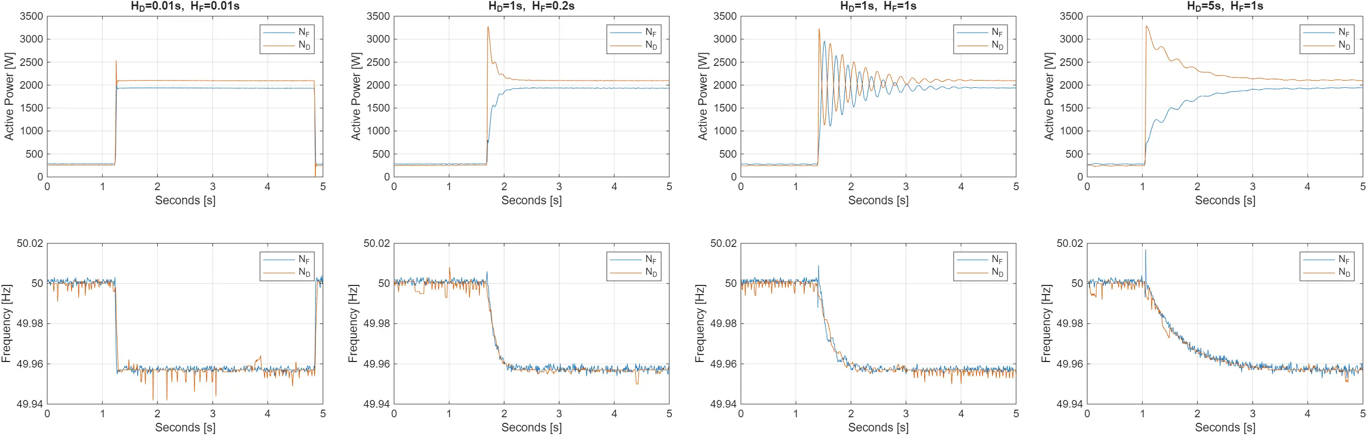 Figure 6: Scenario 1 results with two power converters at nodes \(N_D\) and
\(N_F\) for different levels of synthetic inertia; the 3.5 kW load is at
node \(N_D\).
Figure 6: Scenario 1 results with two power converters at nodes \(N_D\) and
\(N_F\) for different levels of synthetic inertia; the 3.5 kW load is at
node \(N_D\).
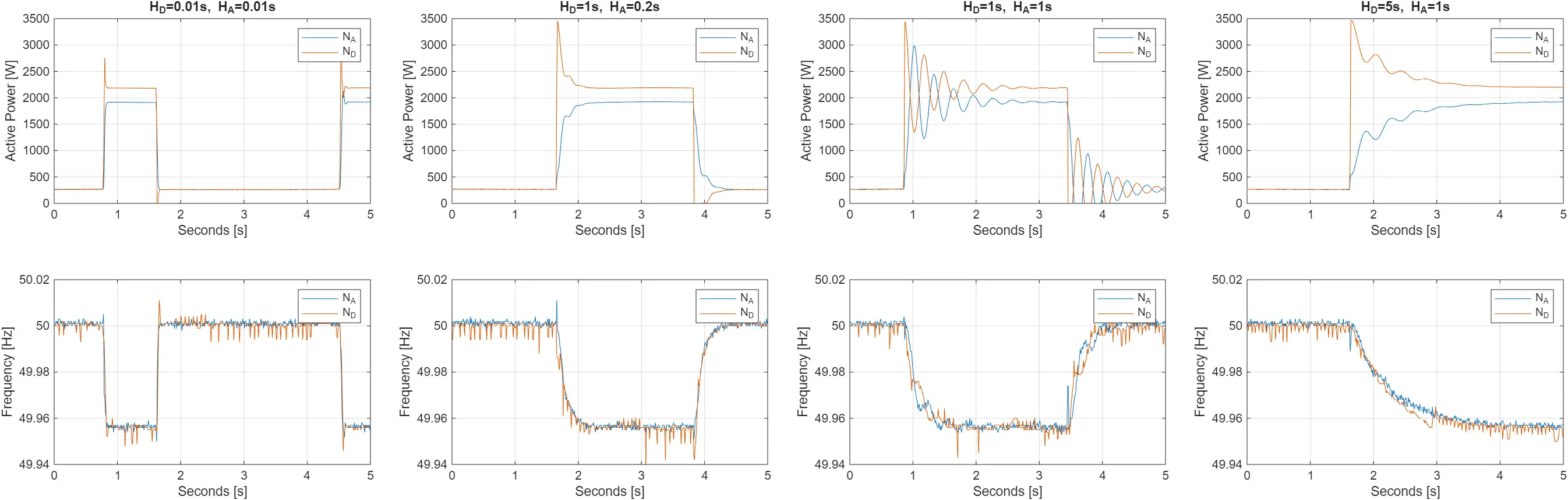 Figure 7: Scenario 2 results with two power converters at nodes \(N_D\) and
\(N_A\) for different levels of synthetic inertia; the 3.5 kW load is at
node \(N_D\).
Figure 7: Scenario 2 results with two power converters at nodes \(N_D\) and
\(N_A\) for different levels of synthetic inertia; the 3.5 kW load is at
node \(N_D\).
When inertia is negligible (both converters at \(H = 0.01\ \text{s}\)), the power is shared rapidly and equally between the two sources (identical droop coefficients). The new frequency setpoint defined by droop control is reached almost immediately, resulting in a high RoCoF of approximately 1 Hz/s. A higher transient power peak is observed in the converter located at the same node (\(N_D\)) as the load.
When inertia is higher (second column of Figures 6 and 7), the RoCoF is considerably lower, around 0.2 Hz/s.
In the third column (both converters at \(H = 1\ \text{s}\)), a frequency swinging phenomenon appears. Comparing the two scenarios, the oscillation appears better damped in the grid with longer lines than in the one with shorter lines — unlike in transmission grids, this behaviour may be attributed to the predominantly resistive nature of distribution lines.
In the fourth and final column, the inertia of the two converters is very different (\(H_D = 5\ \text{s}\) and \(H_F = H_A = 1\ \text{s}\)). The oscillatory phenomenon almost totally disappears, due to the presence of a dominant mass in the system; the converter closer to the load supplies most of the transitory power. The RoCoF is reduced to 0.05 Hz/s.
Regarding steady-state behaviour, in all four inertia settings and under both test scenarios, the power sharing between the converters remains equal, reflecting their identical droop coefficients.
General observation
Whenever the inertia values of the two identical converters are within the same range, power oscillations are observed following the load steps.
3.3 Low-inertia grid: synchronous generator and two GFM converters#
We now reproduce a low-inertia microgrid by activating a synchronous generator within the grid. The generator is connected to node \(N_D\), and the two power converters to nodes \(N_D\) and \(N_F\) respectively, with a varying range of virtual inertia from 0.01 s to 5 s. To illustrate the system dynamics, a 3.5 kW load step is applied at node \(N_D\).
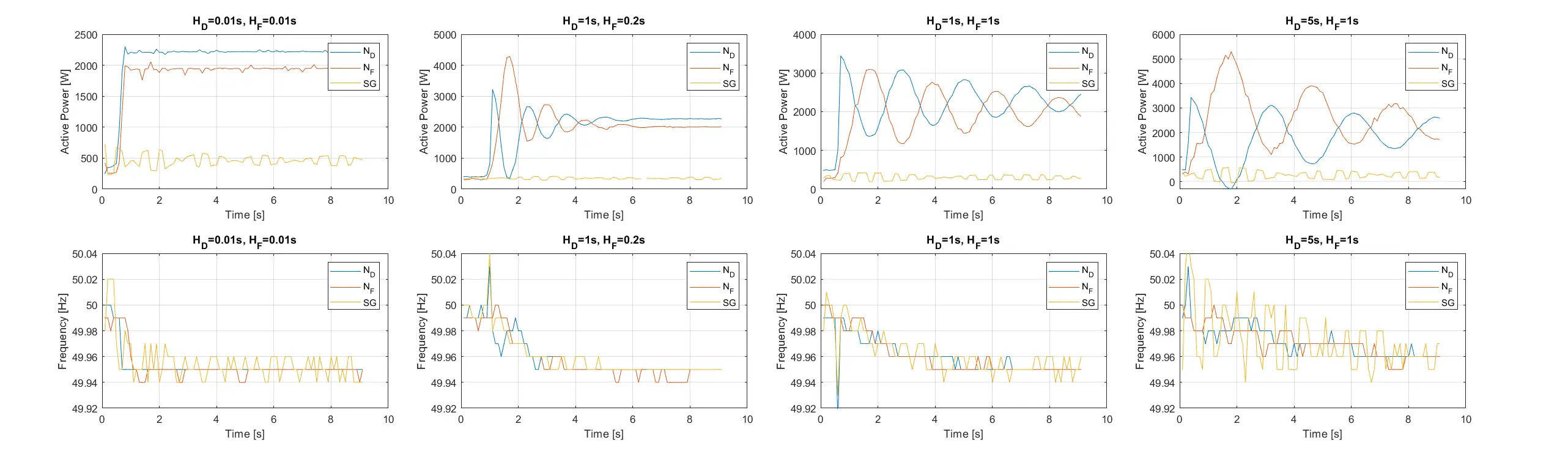 Figure 8: Scenario 1 with two power converters at nodes \(N_D\) and \(N_F\), a
3.5 kW resistive load at node \(N_D\), and a synchronous generator at
node \(N_D\).
Figure 8: Scenario 1 with two power converters at nodes \(N_D\) and \(N_F\), a
3.5 kW resistive load at node \(N_D\), and a synchronous generator at
node \(N_D\).
The configuration with both converters at negligible virtual inertia (\(H = 0.01\ \text{s}\)) is shown in the first column of Figure 8: similarly to the all-converter case, the response of the system is immediate, the power demanded by the load is immediately provided by the two converters according to their droop factor, and no power oscillation is observed.
In the second column (converter at \(N_D\) with \(H_D = 1\ \text{s}\), at \(N_F\) with \(H_F = 0.2\ \text{s}\)), a power oscillation between the two converters appears, with a peak value of double the stationary load. This oscillation is also observed at the inertia values shown in the third and fourth columns. While in the previous test (i.e. with power converters only) the oscillation could be mitigated by assigning different inertia values to the two converters, the current scenario offers less flexibility — the inertia of the synchronous generator cannot be modified. Consequently, when the inertia of any power converter is set to a value similar to that of the generator (~0.5 s), oscillations emerge.
It is worth highlighting that the power-sharing contribution from the generator’s droop controller is not visible in the figure, due to the slow dynamics of the plant’s governor.
3.4 Low-inertia grid: synchronous generator’s governor effect#
As observed above, during a load transient, the synchronous generator contributes minimally to power delivery in the initial moments following the load step. This is primarily due to the slow response of the governor, which delays the generator’s power output. Over time, however, the synchronous generator gradually contributes according to its 5 % droop setting.
This behaviour is illustrated in Figure 9, where a 3.5 kW load step is applied. The converter at node \(N_F\) responds immediately, supplying the required energy from the onset of the transient.
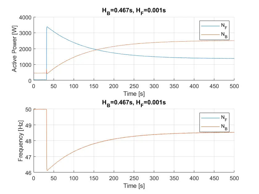 Figure 9: Scenario 2 with one power converter at node \(N_F\), synchronous
generator at node \(N_B\), and load at node \(N_D\).
Figure 9: Scenario 2 with one power converter at node \(N_F\), synchronous
generator at node \(N_B\), and load at node \(N_D\).
In contrast to the experiment in §3.3 (with two converters and one synchronous machine), a slight contribution from the synchronous generator at the moment of the load step is visible — magnified in Figure 10.
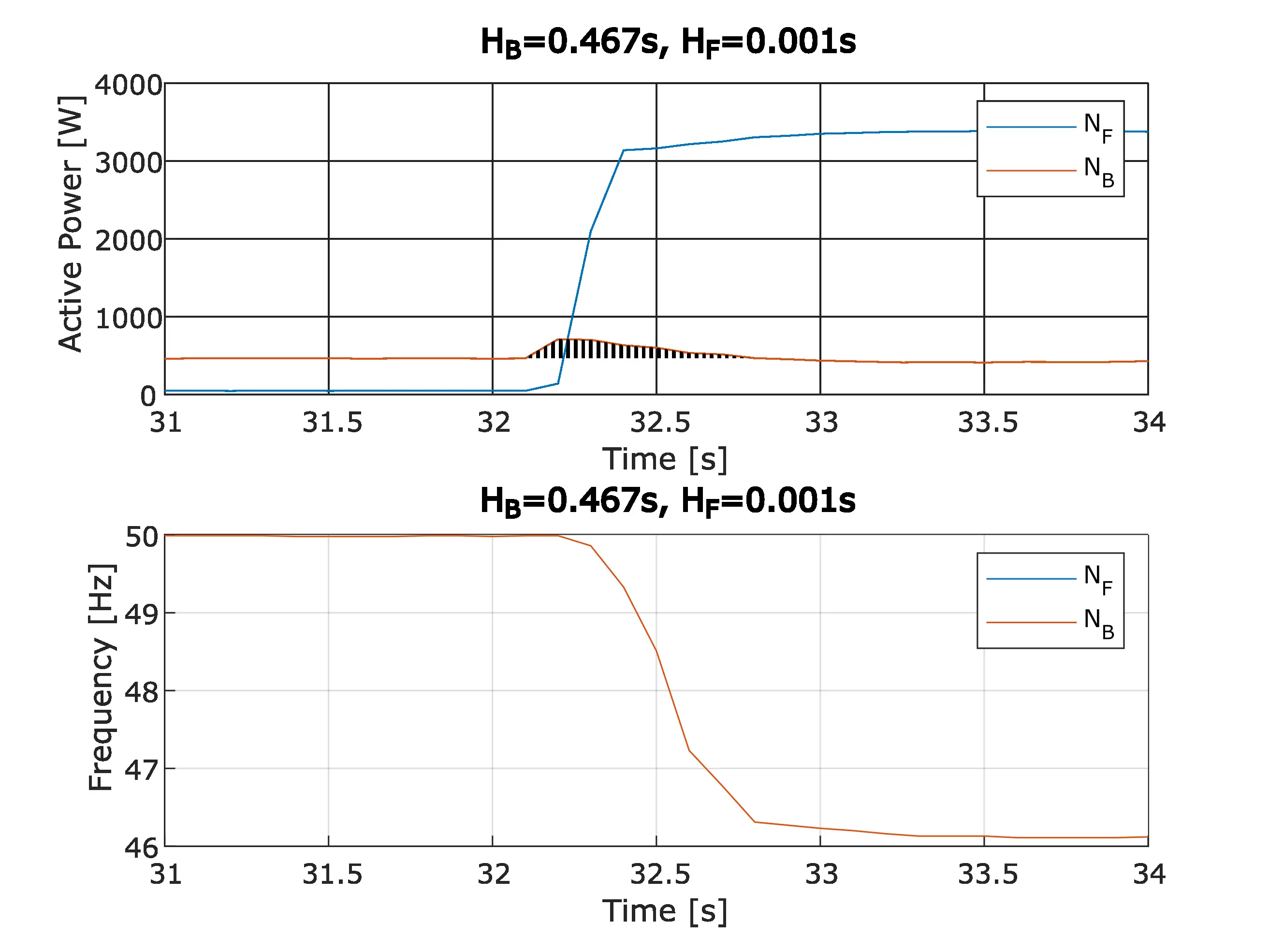 Figure 10: Scenario 2 with one power converter at \(N_F\), synchronous
generator at \(N_B\); 3.5 kW load at \(N_D\), magnified view.
Figure 10: Scenario 2 with one power converter at \(N_F\), synchronous
generator at \(N_B\); 3.5 kW load at \(N_D\), magnified view.
Immediately after the load step, the frequency drops sharply from 50 Hz to 46 Hz, with a maximum RoCoF of approximately 10 Hz/s. This occurs because the inertia of the converter at node \(N_F\) is set very low (\(H_F = 0.001\ \text{s}\)), and it is ultimately the converter’s droop coefficient that halts the frequency decline once the converter fully supplies the transient load.
As a result of this frequency drop, the kinetic energy of the synchronous generator decreases. The difference in kinetic energy is computed (taking into account that the synchronous generator has two poles, \(p = 2\)):
In the magnified Figure 10, the deviation of the active power at node \(N_B\) reflects the effect of the change in kinetic energy, with the hatched area representing the energy exchanged during the transient: \(\Delta E_{\text{elec}} = 101.5\ \text{J}\). The match between \(\Delta E_{\text{elec}}\) and \(\Delta E_{\text{kin}}\) validates the hypothesis that the synchronous generator contributes its kinetic energy.
In the previous test, the virtual inertia of the converter was very low (\(H_F = 0.001\ \text{s}\)). If this virtual inertia is changed to similar values as the synchronous generator, a power oscillation between the two energy sources can be found. In Figure 11, at \(t = 7\ \text{s}\), the virtual inertia of the converter is increased from 0.01 s to 1 s. Even under steady-state conditions, with no applied load step, a power oscillation arises between the converter and the synchronous machine.
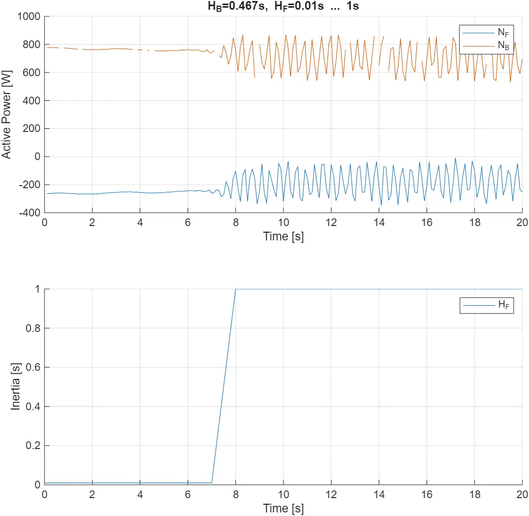 Figure 11: Oscillatory behaviour when approaching similar inertia — ramping
up the virtual inertia in the GFM at \(N_F\) from 0.01 s to 1 s.
Figure 11: Oscillatory behaviour when approaching similar inertia — ramping
up the virtual inertia in the GFM at \(N_F\) from 0.01 s to 1 s.
4. Conclusions#
The effects of the virtual inertia of grid-forming converters are highlighted and contextualized in their interactions with other GFM converters and synchronous machines. The experimental verification of various energy sources within a microgrid has demonstrated the following:
- In microgrids without spinning reserve, converters with similar virtual inertia can lead to power oscillations between the converters. The same behaviour can be observed between synchronous generators and converters: as soon as the inertia is similar, power oscillation can be observed.
- In converter-based microgrids, virtual inertia is indispensable to reduce the RoCoF during transients.
- From a transient perspective, converters located closer to the loads predominantly supply the transient energy. However, in stationary conditions, power distribution aligns with the droop factors of the converters, as expected.
- Droop control without inertia facilitates rapid achievement of new setpoints for both frequency and power. This rapid adjustment results in higher values of RoCoF, which may potentially trigger current protection systems.
In general, when designing the control loop of GFM converters, careful consideration must be given to the other components within the same microgrid. This is crucial because power oscillations can occur during transient events. Control strategies for converters must be carefully coordinated to avoid adverse interactions. Formal stability analyses are currently being conducted to support the experimental results and to incorporate essential elements relevant to real-world implementation and actual hardware.
Acknowledgement
The IT setup adopted in the experimental infrastructure was proposed and validated with the support of Prof. Luca Haab, following the recommendations developed in WP2.